Showcasing AWS Athena

Process your analytical data at very low cost!

In today’s post, I am going to showcase Amazon Athena. Amazon Athena is one of my favourite services within AWS. It has such nice capabilities at a very low cost!

Whether you're a data engineer looking to implement a new analytics solution or a developer seeking to optimize existing Athena workloads, in this post, I will provide insights and examples to help you leverage Athena's full potential.

I hope that after you read this, you have a better understanding on how Athena works. So without further ado, let’s dive in!

If you enjoy this content, take a moment to subscribe; it means a lot to me.

We will not discuss Iceberg in this blog post because I want to cover this topic in detail in a future post about S3 Tables.

What is Amazon Athena

Amazon Athena is an interactive query service that simplifies data analysis in Amazon S3 using standard SQL. Athena is serverless, so there is no infrastructure to set up or manage, and you only pay for the resources your query needs to run.

The above definition is from AWS; believe me, no additional words describe Athena. You put data, catalog data, and query data, and that is it, it is completely serverless (There is a provisioned flavor, but we are not going to dive into this today) without the hassle of spawning up resources, maintaining the cluster, etc.

Athena shines in the following use cases:

• Log analysis and monitoring

• Cost and Usage Analysis

• Data Lake analytics

  • Ad-hoc analysis on a massive amount of data

  • Data processing and cleaning

• Security and compliance

  • Security logs

  • Audit trails

• ML Data Preparation

Athena’s pricing is very straightforward, 5$ per TB of scan, meaning you pay not for compute but based on the amount of data you scanned to generate the required result. You can always use provisioned capacity, but it usually makes sense if you have a large data lake that constantly scans TBs of data. Minimum commitment is 24 DPUs, and a 24/7 usage will cost around 5,000$ per month, so in that case, if you scan more than 1.2PBs per month, provisioned capacity makes sense.

What you’ll learn

This post will show a simple use case on loading, cataloging, and querying data.

We are going to take a look at the following:

• Basics of setting up Amazon Athena

• Configure Athena properly

• Create a Glue crawler for cataloging our Data

• Deploying our IaC in Terraform

This is a Level 200 difficulty, meaning you will need to know some basic concepts of AWS and Terraform

You will need the following:

• An AWS Account and access to credentials of your AWS (either a service account or configure SSO)

• Terraform installed

The whole project will cost approximately: 2-3$

Terraform into Play

For the infrastructure setup, we will create the following resources:

• 2 S3 buckets, one for Athena to save the results and one for sample data

• An Athena workgroup and a database where we will run our queries

• A Glue crawler to catalog our sample data

• IAM policies to provide access

You can find the whole code for this post here, where you can edit the locals.tf file to configure it your way and follow along. So let’s begin, I will showcase some Terraform and explain its usage to make it easier to follow.

First, we need to take a look at the locals.tf file and adjust line 6 and line 17:

• name: add a name for your project, which will be propagated in the resource names

• sample_data_prefix: is the “folder” where we will put the data in S3

Setting up the buckets (main.tf).

module "athena_results_bucket" {
  source  = "terraform-aws-modules/s3-bucket/aws"
  version = "~> 4.8"

  bucket = "${local.name}-query-results"
  force_destroy = true
  acl = "private"

  # Add ownership controls
  control_object_ownership = true
  object_ownership         = "ObjectWriter"

  tags = local.tags
}

# Create a bucket for sample data
module "athena_data_bucket" {
  source  = "terraform-aws-modules/s3-bucket/aws"
  version = "~> 4.8"

  bucket = "${local.name}-data"
  force_destroy = true
  acl = "private"

  # Add ownership controls
  control_object_ownership = true
  object_ownership         = "ObjectWriter"

  tags = local.tags
}

In the code above, we are creating two buckets:

• query-results: Athena needs a bucket to save the generated results in a CSV format and serve them to the user. In this bucket, usually we have a lifecycle policy where we discard the contents after an X number of days.

• data: Athena also needs a bucket where the data is saved and ready for querying. Additionally, Athena can use this bucket to generate data with CTAS statements.

Next, we will create an Athena workgroup and a database to save the data (athena.tf).

resource "aws_athena_workgroup" "athena_workgroup" {
  name        = local.name
  description = "Athena workgroup for ${local.name}"

  configuration {
    enforce_workgroup_configuration    = local.athena_workgroup.enforce_workgroup_configuration
    publish_cloudwatch_metrics_enabled = local.athena_workgroup.publish_cloudwatch_metrics_enabled
    bytes_scanned_cutoff_per_query     = local.athena_workgroup.bytes_scanned_cutoff_per_query

    engine_version {
      selected_engine_version = local.athena_workgroup.engine_version
    }

    result_configuration {
      output_location = "s3://${module.athena_results_bucket.s3_bucket_id}/"

      encryption_configuration {
        encryption_option = local.athena_workgroup.encryption_option
      }
    }
  }

  tags = local.tags
}

resource "aws_athena_database" "athena_database" {
  name   = replace(local.name, "-", "_")
  bucket = module.athena_data_bucket.s3_bucket_id
  force_destroy = true

  properties = {
    location = "s3://${module.athena_data_bucket.s3_bucket_id}/tables/"
  }
} 

You can use Athena workgroups to separate workloads, control team access, enforce configuration, track query metrics, and control costs.

As for the database, we have selected the bucket as our data bucket, but this is primarily for the database metadata. We also defined a location where the data (CTAS) will be saved. We are using force_destroy in case we want to delete the database, avoid this in production workloads.

It is time to create the Glue Crawler to catalog our new data (crawler.tf).

# Create Glue crawler for CUR data
resource "aws_glue_crawler" "demo_crawler" {
  name          = "${local.name}-demo-crawler"
  database_name = aws_athena_database.athena_database.name
  role          = aws_iam_role.glue_crawler.arn
  table_prefix  = "demo_"  # This will prefix all tables created by this crawler

  s3_target {
    path = "s3://${module.athena_data_bucket.s3_bucket_id}/${local.sample_data_prefix}"
  }

  schema_change_policy {
    delete_behavior = "LOG"
    update_behavior = "UPDATE_IN_DATABASE"
  }

  configuration = jsonencode({
    Version = 1.0
    CrawlerOutput = {
      Partitions = { AddOrUpdateBehavior = "InheritFromTable" }
      Tables     = { AddOrUpdateBehavior = "MergeNewColumns" }
    }
  })

  tags = local.tags
} 

The above Terraform code is pretty standard for a Glue Crawler. The most important parts here are:

• s3_target: where we are pointing to the data we have uploaded (not done that yet)

• schema_change_policy: where we provide the behaviour of the catalog when the schema changes, here we say to update the database, but also keep the existing schema on the catalog

Last but not least, we have the IAM policies and roles (iam.tf). There is not much to say here.

Once we are ready, we can proceed with

terraform plan

and once we validate the plan, we can run

terraform apply

And voila! You have a working environment to start putting data and experimenting!

Using Athena

Now that everything is ready, we can populate our S3 bucket with some data. Our choice will be parquet format, and we will upload the iconic Titanic Dataset, which you can find in the repo.

So, navigate to your S3 bucket and upload the dataset under the prefix (data) you have selected above while creating the Glue Crawler. I will use a CLI command, but you are more than welcome to use the console.

aws s3 cp titanic.parquet s3://<bucket_name>/data/titanic.parquet

Then we go to our newly generated crawler and run it to catalog our file. Again, I will use a CLI command.

aws glue start-crawler --name <crawler-name>

This will create a table within our database in Amazon Athena.

We can now run a simple query on our Athena Interface. Use your database name in your case.

SELECT * FROM "thelastdev_athena_demo"."demo_data" limit 10;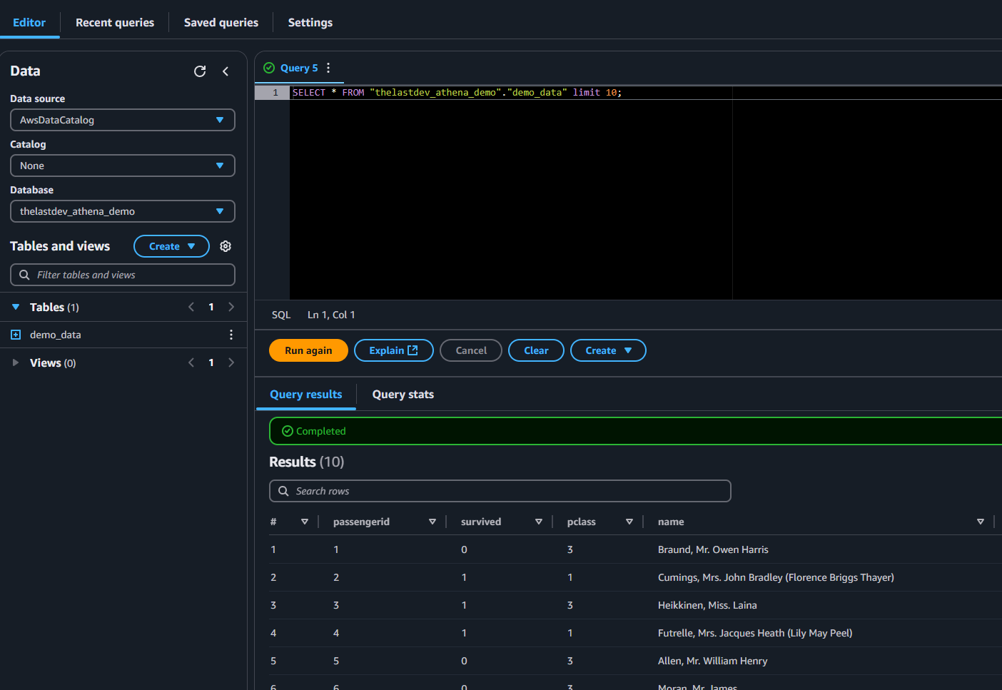

And, believe it or not, this is pretty much it…. This is how Athena works. You can expand your knowledge with the AWS Documentation regarding Athena or by asking Q Developer for more complex implementations.

Closing this post, I will share my notes regarding optimizing Athena.

Athena Optimizations

When it comes to Optimizations, we are going to talk about:

• Cost Optimizations

• Performance Optimizations

So, let’s begin and see the low-hanging fruits:

Partitioning strategies

By properly partitioning your data, you will significantly benefit both in cost and performance optimization. If you utilize a partition in your query (where statement on that field), Athena will only scan the data existing in this partition.

For example, (let’s exaggerate) let’s say you have a bucket with log data going back 3 years, totaling 970 TBs, and the bucket is split into partitions by week. If you search for a specific week or a collection of weeks, Athena will only scan the data and not the 970 TBs to find your results.

To utilize partitioning, you can split your data into prefixes (“folders”) within your bucket

# with one partition
data/week=1/test.parquet
data/week=2/test2.parquet

or

# with multiple partitions
data/year=2025/week=1/day=1/test.partquet

File format selection (Parquet, ORC)

Utilizing a proper format for your data is very very crucial. I personally prefer parquet due to its columnar representation, which allows me to be optimal in select statements (and not *). The difference between CSV files and Parquet regarding performance is significant! Additionally, especially in the CSV format, Athena will open the entire file, while in Parquet, it will be more cost optimized due to its columnar format.

Compression techniques

Because Athena charges you by the amount of TBs you scan, compressing your data will result in lower costs, but not necessarily better performance. My favourite is snappy, fast, and lightweight.

Result caching

You can reuse query results in Athena. When you enable result reuse for a query, Athena looks for a previous query execution within the same workgroup. If Athena finds corresponding stored query results, it does not rerun the query, but points to the previous result location or fetches data from it.

Now, let’s move to more complex optimizations and focus on the 20% of the 80/20 rule. Trying to reach almost optimal performance and cost, but with more effort than the low-hanging fruits we mentioned before.

Query planning - Explain

You can analyze your query execution and discover how Athena scans your data for further optimization.

Workgroup configurations

Cost control settings: You can limit the amount of data that can be scanned in a single query

Performance settings: Use engine version “Athena version 3”, which is currently the latest, but make sure you check the benefits when a new engine comes out.

Publish metrics in CloudWatch to properly monitor Athena usage.

You can see Athena in action with read data in my AWS CUR processing post!

Conclusion

And this is it, this is Amazon Athena. A very powerful and cheap database where you can query your structured and semi-structured data. As a next step, I will go through the S3 Tables to see Athena in action with Iceberg, and move on to the remaining data stack of AWS, like AWS Glue Jobs, Lake Formation, Redshift, and many more.

Feel free to reach out if you encounter any problems or have suggestions.

Till the next time, stay safe and have fun!

If you enjoy this content, take a moment to subscribe; it means a lot to me.